Ellipsoid modelling for calibration purposes

Magnetometers are highly sensitive to local deviations of the magnetic field, affecting the desired measurement of the Earth geomagnetic field. Triaxial accelerometers, however, can have slight offsets in and misalignments of their axes which need to be corrected to properly interpret their output. One commonly used method for performing these corrections is done by fitting an ellipsoid model to data collected while the sensor’s axes are exposed to the forces of the fields they measure.

# Set up
import importlib.resources as rsrc
import xarray as xr
import numpy as np
import matplotlib.pyplot as plt
import skdiveMove.imutools as imutools
from mpl_toolkits.mplot3d import Axes3D

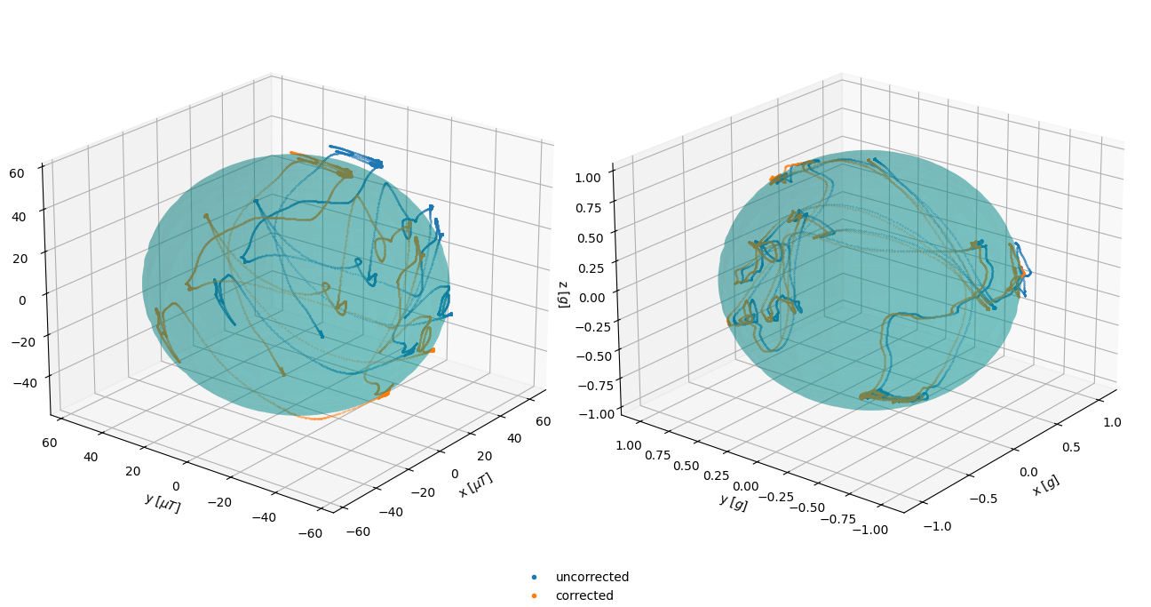
To demonstrate this procedure with utilities from the allan submodule, measurements from a triaxial accelerometer and magnetometer were recorded at 100 Hz sampling frequency with an IMU that was rotated around the main axes to cover a large surface of the sphere.

icdf = (rsrc.files("skdiveMove") / "tests" / "data" /
        "gertrude" / "magnt_accel_calib.nc")
magnt_accel = xr.load_dataset(icdf)
magnt = magnt_accel["magnetic_density"].to_numpy()
accel = magnt_accel["acceleration"].to_numpy()

The function imutools.fit_ellipsoid() returns the offset, gain, and rotation matrix (if requested) necessary to correct the sensor’s data. There are six types of constraint to impose on the result, including which radii should be equal, and whether the data should be rotated.

# Here, a symmetrical constraint whereby any plane passing through the
# origin is used, with all radii equal to each other
magnt_off, magnt_gain, _ = imutools.fit_ellipsoid(magnt, f="sxyz")
accel_off, accel_gain, _ = imutools.fit_ellipsoid(accel, f="sxyz")

Inspect the offsets and gains in the uncorrected data:

Magnetometer offsets [uT]: x=13.46, y=-7.55, z=9.68; gains [uT]: x=48.67, y=48.67, z=48.67
Accelerometer offsets [g]: x=0.027, y=-0.031, z=0.007; gains [g]: x=1.001, y=1.001, z=1.001

Calibrate the sensors using these estimates:

magnt_refr = 56.9
magnt_corr = imutools.apply_ellipsoid(magnt, offset=magnt_off,
                                      gain=magnt_gain,
                                      rotM=np.diag(np.ones(3)),
                                      ref_r=magnt_refr)
accel_corr = imutools.apply_ellipsoid(accel, offset=accel_off,
                                      gain=accel_gain,
                                      rotM=np.diag(np.ones(3)),
                                      ref_r=1.0)

An appreciation of the effect of the calibration can be observed by comparing the difference between maxima/minima and the reference value for the magnetic field at the geographic location and time of the measurements, or 1 $g$ in the case of the accelerometers.

magnt_refr_diff = [np.abs(magnt.max(axis=0)) - magnt_refr,
                   np.abs(magnt.min(axis=0)) - magnt_refr]
magnt_corr_refr_diff = [np.abs(magnt_corr.max(axis=0)) - magnt_refr,
                        np.abs(magnt_corr.min(axis=0)) - magnt_refr]

accel_refr_diff = [np.abs(accel.max(axis=0)) - 1.0,
                   np.abs(accel.min(axis=0)) - 1.0]
accel_corr_refr_diff = [np.abs(accel_corr.max(axis=0)) - 1.0,
                        np.abs(accel_corr.min(axis=0)) - 1.0]

Uncorrected magnetometer difference to reference [uT]:
maxima: x=5.78, y=-17.06, z=2.24; minima: x=-24.07, y=-0.56, z=-19.21
Corrected magnetometer difference to reference [uT]:
maxima: x=0.64, y=-1.51, z=0.91; minima: x=-2.78, y=0.14, z=-1.52
Uncorrected accelerometer difference to reference [g]:
maxima: x=0.06, y=-0.01, z=0.02; minima: x=0.01, y=0.03, z=0.02
Corrected accelerometer difference to reference [g]:
maxima: x=0.04, y=0.02, z=0.01; minima: x=0.04, y=-0.00, z=0.03

Or compare visually on a 3D plot:

Feel free to download a copy of this demo (demo_ellipsoid.py).